WARNING
Interactive examples are a work in progress for this page.
Spatial autocorrelation statistics
By Omar Kawach
What is spatial autocorrelation statistics?
Spatial autocorrelation statistics in geographic information systems (GIS) assess relationships between variable values at different locations, measuring similarity or dissimilarity based on distance. They identify patterns like clustering or dispersion, aiding fields such as environmental science, urban planning, and epidemiology. For example, if the values of a variable are clustered together in one area and dispersed in another, this may indicate a relationship between the variable and other spatial factors, such as socioeconomic status or natural resources.
Types of spatial autocorrelation statistics
There are two main types of spatial autocorrelation statistics: global statistics and local statistics. Global statistics, like Global Moran's I, summarize the overall pattern of spatial autocorrelation in a dataset. In contrast, local statistics, such as Local Moran's I, provide information on the spatial autocorrelation of values within specific geographic areas.
Considerations
Spatial autocorrelation statistics follow Tobler's first law of Geography (TFL) where near things are more related than distant things. When conducting statistical analysis, the outcome of the correlation coefficient from Moran's I can explain the relationship between two values (or multiple locations). The relationship between two values (bivariate) can either be by chance or correlated. This is where you would reject or accept a hypothesis and show that the distribution is/isn't random, which is the same as cause and effect in data.
Moran's I
Moran's I generally describes a measure of spatial autocorrelation, indicating the degree to which a set of spatial data points are clustered, dispersed, or randomly distributed. Global Moran's I measures how clustered or dispersed values are in a dataset/study area. Local Moran's I can be used to identify specific spatial clusters or outliers within a dataset.
In the formula for Moran's I, ( N ) represents the number of regions or spatial units, and ( W ) represents the sum of all weights. There are different weight matrices such as queen contiguity, rook contiguity, distance, and k-nearest neighbors.
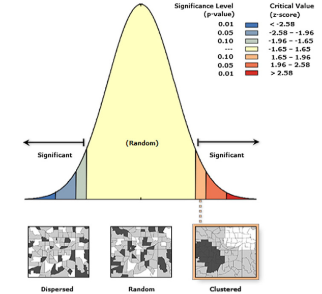
The output of Moran's I ranges between -1 and +1, where a positive value indicates similar values are found together, a negative value (which is rare) indicates dissimilar values are found together, and a value of 0 means the distribution is random with no spatial autocorrelation.
Additionally, measuring significance is important, as p-values determine the probability of spatial autocorrelation/null hypothesis being true, and z-scores indicate the likelihood that the data is spatially autocorrelated. You can calculate the p-value by comparing random distributions of data to the observed data (a low p-value is desirable), and the z-score by comparing the observed data to the mean and standard deviation of the random distributions (a high absolute value is desirable).
Distance decay is another factor to consider, as Moran's I decreases when more distant observations are included in the calculations, thus having less influence.
Local indicators of spatial association (LISA)
A LISA cluster map uses Local Moran's I to inform where things are concentrated (hot spot, relationship likely not by chance) and where they are not (cold spot). Spatial clusters in LISA indicate areas where similar values (high or low) are grouped together, while spatial outliers highlight areas where a value significantly differs from its surrounding values.
Spatial clusters
- high high (red) indicates a high concentration within itself and surrounding areas
- low low (blue) indicates a low concentration when surrounding areas have more concentration
Spatial outliers
- high low (light red) indicates a high concentration when surrounding areas have low conc
- low high (light blue) indicates a low concentration when surrounding areas have high conc
Spatiotemporal dependence (space and time)
The two most challenging aspects of spatial statistics, or GIS in general, are space and time. Consider that the weather at one location is likely to be similar to the weather of a nearby location, but the weather at both locations is also likely to change over time. Spatiotemporal dependence combines both spatial dependence and temporal dependence. Spatial dependence signifies that values of a variable at one location can depend on values of that same variable at other locations. It's worth mentioning that there are issues related to spatial dependance that impact statistical tests:
- Modifiable Areal Unit Problem (MAUP) can introduce bias
- Boundaries impact statistical tests (most importantly, look at standard deviation)
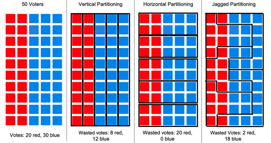
- Location of boundaries used to aggregate data can influence results of statistical tests (Moran's I)
- Gerrymandering is a good example of this
- Ecological fallacy can result in weak inferences
- Individuals vs populations
- Cant take aggregated results and apply them to individuals
- Statistical test results change based on data aggregation
- Sampling methods such as random, stratified random, and systematic sampling can dictate sampling bias
- For a good amount of spatial representation and to avoid bias, use stratified random sampling
- Boundary problem might lead to loss of information
Interaction
Coming soon
Test your knowledge
Gerrymandering is an example of which type of spatial analysis?


